Introduction
The single-cell
integration benchmarking (scIB) project was an effort to evaluate
and compare the performance of methods for integrating single-cell RNA
and ATAC sequencing datasets (Luecken et al.
2021). Many of the results were displayed using custom scripts to
create visualisations similar to those produced by
funkyheatmap.
In this vignette we will show how these figures can be reproduced
using funkyheatmap.
Summary figure
The first figure we will recreate is the summary figure showing the performance of all methods on RNA data. Here is the original for reference:

scIB RNA summary figure
Data
The steps for summarising the raw metric scores are quite complex so
we have included a pre-processed summary table as part of
funkyheatmap which is produced from the files available in
the scIB
reproducibility repository.
data("scib_summary")
glimpse(scib_summary)
#> Rows: 20
#> Columns: 27
#> $ method                      <chr> "scANVI*", "Scanorama", "scVI", "FastMNN",…
#> $ output                      <chr> "Embedding", "Embedding", "Embedding", "Em…
#> $ features                    <chr> "HVG", "HVG", "HVG", "HVG", "HVG", "HVG", …
#> $ scaling                     <chr> "Unscaled", "Scaled", "Unscaled", "Unscale…
#> $ avg_rank                    <dbl> 4.6, 8.0, 9.4, 10.4, 13.2, 13.2, 18.0, 21.…
#> $ overall_immune_cell_hum     <dbl> 0.8217139, 0.8484369, 0.7880395, 0.8456189…
#> $ overall_immune_cell_hum_mou <dbl> 0.6275154, 0.6415929, 0.6367120, 0.6049282…
#> $ overall_lung_atlas          <dbl> 0.7557935, 0.7088485, 0.7196019, 0.7083853…
#> $ overall_mouse_brain         <dbl> 0.7331990, 0.6725443, 0.6773415, 0.6062384…
#> $ overall_pancreas            <dbl> 0.7238847, 0.7034837, 0.7134047, 0.7200626…
#> $ overall_simulations_1_1     <dbl> 0.8528483, 0.8522969, 0.8141741, 0.7446178…
#> $ overall_simulations_2       <dbl> 0.7365843, 0.5265792, 0.5022136, 0.7052069…
#> $ rank_immune_cell_hum        <dbl> 4, 1, 14, 2, 5, 7, 10, 21, 20, 47, 48, 19,…
#> $ rank_immune_cell_hum_mou    <dbl> 4.0, 2.0, 3.0, 9.0, 25.0, 1.0, 15.0, 33.0,…
#> $ rank_lung_atlas             <dbl> 3.0, 6.0, 5.0, 7.0, 28.0, 2.0, 15.0, 23.0,…
#> $ rank_mouse_brain            <dbl> 1, 10, 9, 21, 7, 50, 27, 12, 50, 2, 6, 50,…
#> $ rank_pancreas               <dbl> 11, 21, 16, 13, 1, 6, 23, 17, 2, 14, 33, 4…
#> $ rank_simulations_1_1        <dbl> 3, 4, 13, 35, 38, 23, 46, 25, 57, 53, 21, …
#> $ rank_simulations_2          <dbl> 4, 25, 28, 6, 8, 2, 12, 23, 61, 19, 26, 20…
#> $ package_score               <dbl> 0.8102822, 0.7686694, 0.8831989, 0.7993550…
#> $ package_rank                <dbl> 7.0, 10.0, 5.0, 8.0, 6.0, 12.0, 8.0, 10.0,…
#> $ paper_score                 <dbl> 0.43750, 0.87500, 0.65625, 0.25000, 1.0000…
#> $ paper_rank                  <dbl> 14.5, 5.0, 12.0, 16.0, 1.5, 13.0, 16.0, 5.…
#> $ time_score                  <dbl> 0.5540645, 0.6355258, 0.5682302, 0.6434753…
#> $ time_rank                   <dbl> 36, 17, 28, 16, 10, 50, 16, 17, 32, 3, 2, …
#> $ memory_score                <dbl> 0.4905173, 0.4046461, 0.5201664, 0.4347876…
#> $ memory_rank                 <dbl> 3, 21, 1, 14, 10, 22, 14, 21, 45, 2, 11, 1…
This data frame contains several columns: details of the method version and output, an average rank used to order the table, overall scores and ranks for the performance on each dataset, usability scores and ranks (for the package and paper), and scalability scores and ranks (for both time and memory). All of these will go into the summary table.
The dataset requires some preparation for the
funky_heatmap() function. We will create an id
column using the row numbers (the data is already sorted by performance
ranking). We also create label columns for each of the scores showing
the top 3 performers and relabel some of the columns. Finally, we subset
to a the set of columns we want to plot.
# A small helper function for creating rank labels for each column.
# It takes a scores, ranks them and returns a character vector with labels for
# the top 3 scores. Any additional arguments are passed to the `rank()`
# function.
label_top_3 <- function(scores, ...) {
  ranks <- rank(scores, ...)
  ifelse(ranks <= 3, as.character(ranks), "")
}

scib_summary_plot <- scib_summary |>
  # Create an ID column showing the final rank
  mutate(id = as.character(seq_len(nrow(scib_summary)))) |>
  # Set the labels for the scaling and features columns
  mutate(
    scaling = factor(
      scaling,
      levels = c("Unscaled", "Scaled"),
      labels = c("-", "+")
    ),
    features = factor(
      features,
      levels = c("Full", "HVG"),
      labels = c("FULL", "HVG")
    )
  ) |>
  # Create a column with paths to output images
  mutate(
    output_img = case_match(
      output,
      "Features"  ~ "images/matrix.png",
      "Embedding" ~ "images/embedding.png",
      "Graph"     ~ "images/graph.png"
    )
  ) |>
  # Create rank labels
  mutate(
    label_pancreas = label_top_3(rank_pancreas),
    label_lung_atlas = label_top_3(rank_lung_atlas),
    label_immune_cell_hum = label_top_3(rank_immune_cell_hum),
    label_immune_cell_hum_mou = label_top_3(rank_immune_cell_hum_mou),
    label_mouse_brain = label_top_3(rank_mouse_brain),
    label_simulations_1_1 = label_top_3(rank_simulations_1_1),
    label_simulations_2 = label_top_3(rank_simulations_2),
    package_label = label_top_3(package_rank, ties.method = "min"),
    paper_label = label_top_3(paper_rank, ties.method = "min"),
    time_label = label_top_3(time_rank, ties.method = "min"),
    memory_label = label_top_3(memory_rank, ties.method = "min")
  ) |>
  # scale rank columns between [0, 1] because `scale_column` is set to FALSE.
  mutate_at(
    c("rank_pancreas", "rank_lung_atlas", "rank_immune_cell_hum", "rank_immune_cell_hum_mou", "rank_mouse_brain", "rank_simulations_1_1", "rank_simulations_2", "package_rank", "paper_rank", "time_rank", "memory_rank"),
    function(x) { scale_minmax(-x) }
  ) |>
  as.data.frame()

glimpse(scib_summary_plot)
#> Rows: 20
#> Columns: 40
#> $ method                      <chr> "scANVI*", "Scanorama", "scVI", "FastMNN",…
#> $ output                      <chr> "Embedding", "Embedding", "Embedding", "Em…
#> $ features                    <fct> HVG, HVG, HVG, HVG, HVG, HVG, HVG, HVG, HV…
#> $ scaling                     <fct> -, +, -, -, -, -, -, +, +, -, -, +, -, -, …
#> $ avg_rank                    <dbl> 4.6, 8.0, 9.4, 10.4, 13.2, 13.2, 18.0, 21.…
#> $ overall_immune_cell_hum     <dbl> 0.8217139, 0.8484369, 0.7880395, 0.8456189…
#> $ overall_immune_cell_hum_mou <dbl> 0.6275154, 0.6415929, 0.6367120, 0.6049282…
#> $ overall_lung_atlas          <dbl> 0.7557935, 0.7088485, 0.7196019, 0.7083853…
#> $ overall_mouse_brain         <dbl> 0.7331990, 0.6725443, 0.6773415, 0.6062384…
#> $ overall_pancreas            <dbl> 0.7238847, 0.7034837, 0.7134047, 0.7200626…
#> $ overall_simulations_1_1     <dbl> 0.8528483, 0.8522969, 0.8141741, 0.7446178…
#> $ overall_simulations_2       <dbl> 0.7365843, 0.5265792, 0.5022136, 0.7052069…
#> $ rank_immune_cell_hum        <dbl> 0.95081967, 1.00000000, 0.78688525, 0.9836…
#> $ rank_immune_cell_hum_mou    <dbl> 0.95238095, 0.98412698, 0.96825397, 0.8730…
#> $ rank_lung_atlas             <dbl> 0.9850746, 0.9402985, 0.9552239, 0.9253731…
#> $ rank_mouse_brain            <dbl> 1.0000000, 0.8163265, 0.8367347, 0.5918367…
#> $ rank_pancreas               <dbl> 0.84126984, 0.68253968, 0.76190476, 0.8095…
#> $ rank_simulations_1_1        <dbl> 1.0000000, 0.9848485, 0.8484848, 0.5151515…
#> $ rank_simulations_2          <dbl> 0.9661017, 0.6101695, 0.5593220, 0.9322034…
#> $ package_score               <dbl> 0.8102822, 0.7686694, 0.8831989, 0.7993550…
#> $ package_rank                <dbl> 0.62068966, 0.41379310, 0.75862069, 0.5517…
#> $ paper_score                 <dbl> 0.43750, 0.87500, 0.65625, 0.25000, 1.0000…
#> $ paper_rank                  <dbl> 0.1034483, 0.7586207, 0.2758621, 0.0000000…
#> $ time_score                  <dbl> 0.5540645, 0.6355258, 0.5682302, 0.6434753…
#> $ time_rank                   <dbl> 0.29166667, 0.68750000, 0.45833333, 0.7083…
#> $ memory_score                <dbl> 0.4905173, 0.4046461, 0.5201664, 0.4347876…
#> $ memory_rank                 <dbl> 0.9629630, 0.6296296, 1.0000000, 0.7592593…
#> $ id                          <chr> "1", "2", "3", "4", "5", "6", "7", "8", "9…
#> $ output_img                  <chr> "images/embedding.png", "images/embedding.…
#> $ label_pancreas              <chr> "", "", "", "", "1", "3", "", "", "2", "",…
#> $ label_lung_atlas            <chr> "2", "", "3", "", "", "1", "", "", "", "",…
#> $ label_immune_cell_hum       <chr> "3", "1", "", "2", "", "", "", "", "", "",…
#> $ label_immune_cell_hum_mou   <chr> "", "2", "3", "", "", "1", "", "", "", "",…
#> $ label_mouse_brain           <chr> "1", "", "", "", "", "", "", "", "", "2", …
#> $ label_simulations_1_1       <chr> "1", "2", "", "", "", "", "", "", "", "", …
#> $ label_simulations_2         <chr> "2", "", "", "3", "", "1", "", "", "", "",…
#> $ package_label               <chr> "", "", "", "", "", "", "", "", "1", "", "…
#> $ paper_label                 <chr> "", "", "", "", "1", "", "", "", "", "3", …
#> $ time_label                  <chr> "", "", "", "", "", "", "", "", "", "2", "…
#> $ memory_label                <chr> "3", "", "1", "", "", "", "", "", "", "2",…
Column information
The first step in plotting the figure is to create a data frame describing how we want to plot the columns.
column_info <- tribble(# tribble_start
                              ~id,                   ~id_color,                   ~name,    ~geom,         ~group,                                                      ~options,
                             "id",                          NA,                  "Rank",   "text",       "Method",                                               list(hjust = 0),
                         "method",                          NA,                "Method",   "text",       "Method",                                    list(hjust = 0, width = 5),
                     "output_img",                          NA,                "Output",  "image",       "Method",                                                        list(),
                       "features",                  "features",              "Features",   "text",       "Method",                         list(palette = "features", width = 2),
                        "scaling",                          NA,               "Scaling",   "text",       "Method",                                       list(fontface = "bold"),
               "overall_pancreas",             "rank_pancreas",              "Pancreas",    "bar",          "RNA",    list(palette = "blues", width = 1.5, draw_outline = FALSE),
                 "label_pancreas",                          NA,                      NA,   "text",          "RNA",                              list(hjust = .1, overlay = TRUE),
             "overall_lung_atlas",           "rank_lung_atlas",                  "Lung",    "bar",          "RNA",    list(palette = "blues", width = 1.5, draw_outline = FALSE),
               "label_lung_atlas",                          NA,                      NA,   "text",          "RNA",                              list(hjust = .1, overlay = TRUE),
        "overall_immune_cell_hum",      "rank_immune_cell_hum",        "Immune (human)",    "bar",          "RNA",    list(palette = "blues", width = 1.5, draw_outline = FALSE),
          "label_immune_cell_hum",                          NA,                      NA,   "text",          "RNA",                              list(hjust = .1, overlay = TRUE),
    "overall_immune_cell_hum_mou",  "rank_immune_cell_hum_mou",  "Immune (human/mouse)",    "bar",          "RNA",    list(palette = "blues", width = 1.5, draw_outline = FALSE),
      "label_immune_cell_hum_mou",                          NA,                      NA,   "text",          "RNA",                              list(hjust = .1, overlay = TRUE),
            "overall_mouse_brain",          "rank_mouse_brain",           "Mouse brain",    "bar",          "RNA",    list(palette = "blues", width = 1.5, draw_outline = FALSE),
              "label_mouse_brain",                          NA,                      NA,   "text",          "RNA",                              list(hjust = .1, overlay = TRUE),
        "overall_simulations_1_1",      "rank_simulations_1_1",                 "Sim 1",    "bar",  "Simulations",   list(palette = "greens", width = 1.5, draw_outline = FALSE),
          "label_simulations_1_1",                          NA,                      NA,   "text",  "Simulations",                              list(hjust = .1, overlay = TRUE),
          "overall_simulations_2",        "rank_simulations_2",                 "Sim 2",    "bar",  "Simulations",   list(palette = "greens", width = 1.5, draw_outline = FALSE),
            "label_simulations_2",                          NA,                      NA,   "text",  "Simulations",                              list(hjust = .1, overlay = TRUE),
                  "package_score",              "package_rank",               "Package",    "bar",    "Usability",  list(palette = "oranges", width = 1.5, draw_outline = FALSE),
                  "package_label",                          NA,                      NA,   "text",    "Usability",                              list(hjust = .1, overlay = TRUE),
                    "paper_score",                "paper_rank",                 "Paper",    "bar",    "Usability",  list(palette = "oranges", width = 1.5, draw_outline = FALSE),
                    "paper_label",                          NA,                      NA,   "text",    "Usability",                              list(hjust = .1, overlay = TRUE),
                     "time_score",                 "time_rank",                  "Time",    "bar",  "Scalability",    list(palette = "greys", width = 1.5, draw_outline = FALSE),
                     "time_label",                          NA,                      NA,   "text",  "Scalability",                              list(hjust = .1, overlay = TRUE),
                   "memory_score",               "memory_rank",                "Memory",    "bar",  "Scalability",    list(palette = "greys", width = 1.5, draw_outline = FALSE),
                   "memory_label",                          NA,                      NA,   "text",  "Scalability",                              list(hjust = .1, overlay = TRUE)
) # tribble_end

column_info
#> # A tibble: 27 × 6
#>    id                      id_color             name    geom  group options
#>    <chr>                   <chr>                <chr>   <chr> <chr> <list>
#>  1 id                      NA                   Rank    text  Meth… <named list>
#>  2 method                  NA                   Method  text  Meth… <named list>
#>  3 output_img              NA                   Output  image Meth… <list [0]>
#>  4 features                features             Featur… text  Meth… <named list>
#>  5 scaling                 NA                   Scaling text  Meth… <named list>
#>  6 overall_pancreas        rank_pancreas        Pancre… bar   RNA   <named list>
#>  7 label_pancreas          NA                   NA      text  RNA   <named list>
#>  8 overall_lung_atlas      rank_lung_atlas      Lung    bar   RNA   <named list>
#>  9 label_lung_atlas        NA                   NA      text  RNA   <named list>
#> 10 overall_immune_cell_hum rank_immune_cell_hum Immune… bar   RNA   <named list>
#> # ℹ 17 more rows
As shown in the other vignettes this table includes the type of geom for each each column and how they are grouped as well as some configuration options for how they are displayed. Note that we overlay the labels for each score over the corresponding bars.
We also describe the various column groups.
column_groups <- tribble(
        ~ group,     ~ palette,      ~ level1,
       "Method",       "black",      "Method",
          "RNA",       "blues",         "RNA",
  "Simulations",      "greens", "Simulations",
    "Usability",     "oranges",   "Usability",
  "Scalability",       "greys", "Scalability",
)

column_groups
#> # A tibble: 5 × 3
#>   group       palette level1
#>   <chr>       <chr>   <chr>
#> 1 Method      black   Method
#> 2 RNA         blues   RNA
#> 3 Simulations greens  Simulations
#> 4 Usability   oranges Usability
#> 5 Scalability greys   Scalability
There isn’t much customisation here, we are mostly just defining the labels for each group.
Row information
We aren’t applying any grouping to the rows so the row information is very basic.
row_info <- data.frame(id = scib_summary_plot$id, group = NA_character_)

row_info
#>    id group
#> 1   1  <NA>
#> 2   2  <NA>
#> 3   3  <NA>
#> 4   4  <NA>
#> 5   5  <NA>
#> 6   6  <NA>
#> 7   7  <NA>
#> 8   8  <NA>
#> 9   9  <NA>
#> 10 10  <NA>
#> 11 11  <NA>
#> 12 12  <NA>
#> 13 13  <NA>
#> 14 14  <NA>
#> 15 15  <NA>
#> 16 16  <NA>
#> 17 17  <NA>
#> 18 18  <NA>
#> 19 19  <NA>
#> 20 20  <NA>
Palettes
The palettes are mostly the default palettes, with the addition of the features, oranges and black palettes.
palettes <- list(
  features = c(FULL = "#4c4c4c", HVG = "#006300"),
  blues = "Blues",
  greens = "Greens",
  oranges = rev(RColorBrewer::brewer.pal(9, "Oranges")),
  greys = "Greys",
  black = c("black", "black")
)
Legends
legends <- list(
  list(
    title = "Scaling",
    geom = "text",
    values = c("Scaled", "Unscaled"),
    labels = c("+", "-"),
    label_width = .5
  ),
  list(
    title = "RNA rank",
    palette = "blues",
    geom = "rect",
    labels = c("20", " ", "10", " ", "1"),
    size = c(1, 1, 1, 1, 1)
  ),
  list(
    title = "Simulations rank",
    palette = "greens",
    geom = "rect",
    labels = c("20", " ", "10", " ", "1"),
    size = c(1, 1, 1, 1, 1)
  ),
  list(
    title = "Usability rank",
    palette = "oranges",
    geom = "rect",
    labels = c("20", " ", "10", " ", "1"),
    size = c(1, 1, 1, 1, 1)
  ),
  list(
    title = "Scalability rank",
    palette = "greys",
    geom = "rect",
    labels = c("20", " ", "10", " ", "1"),
    size = c(1, 1, 1, 1, 1)
  )
)
Figure
Now that we have defined everything we can make the summary figure.
funky_heatmap(
  data = scib_summary_plot,
  column_info = column_info,
  column_groups = column_groups,
  row_info = row_info,
  palettes = palettes,
  legends = legends,
  position_args = position_arguments(
    col_annot_offset = 4
  ),
  scale_column = FALSE
)
#> ℹ Column info did not contain a column called 'legend', generating options based on the 'geom' column.
#> ℹ Some palettes were not used in the column info, adding legends for them.
#> ℹ Legend 2 did not contain color, inferring from the palette.
#> ℹ Legend 3 did not contain color, inferring from the palette.
#> ℹ Legend 4 did not contain color, inferring from the palette.
#> ℹ Legend 5 did not contain color, inferring from the palette.
#> ℹ Legend 6 did not contain a geom, inferring from the column info.
#> ℹ Legend 6 did not contain labels, inferring from the geom.
#> ! Legend 6 has geom 'text' but no specified labels, so disabling this legend for now.
#> Warning: Removed 12 rows containing missing values (`geom_rect()`).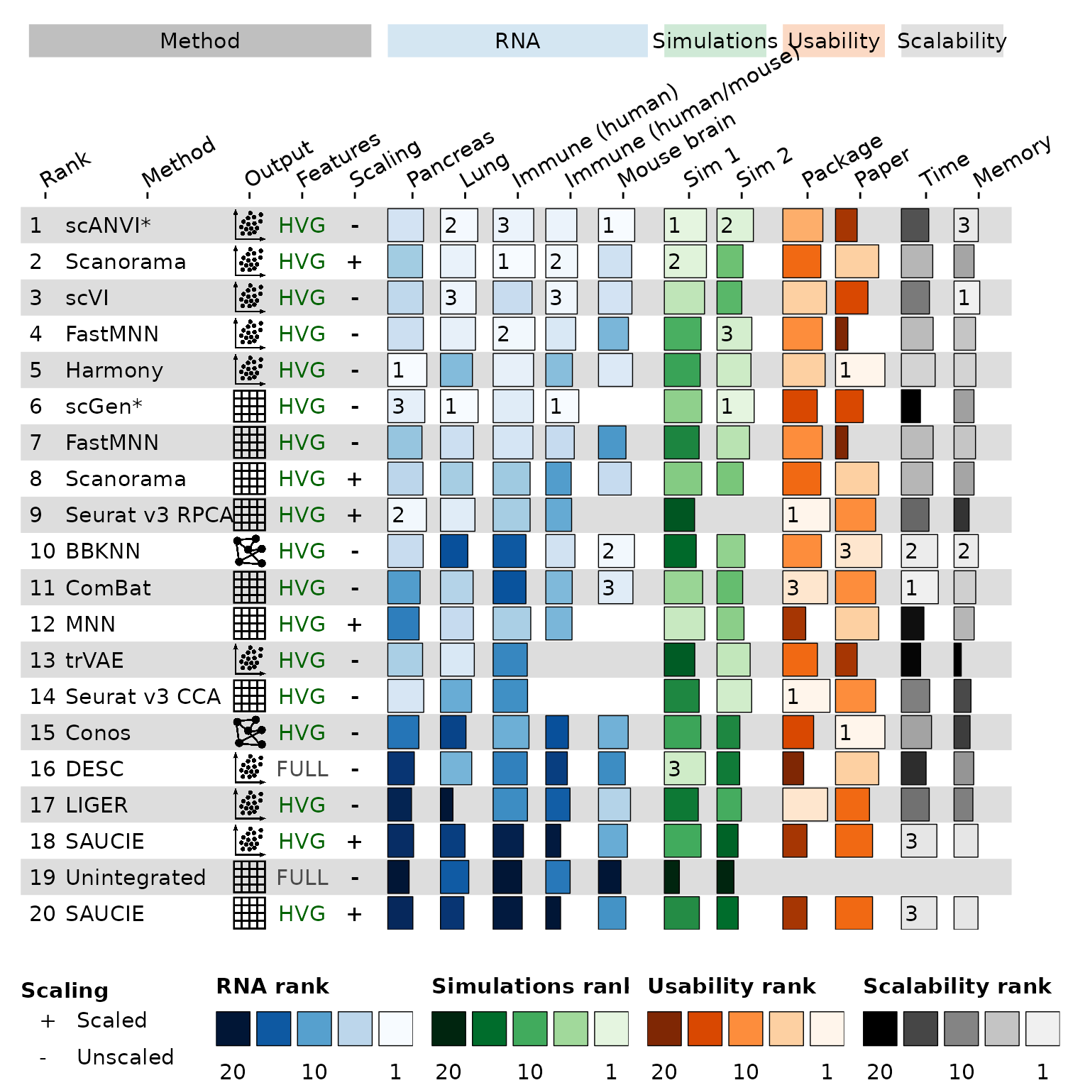
This isn’t exactly like the original figure but it is fairly close. Most of the differences are cosmetic such as alignment of labels and the lack of fancy headings. If you compare closely to the original figure you may also notice some changes in the method ranking compared to the original figure due to small difference in the pre-processing of the raw data.